Photometry: Measuring the Stars

Light from the stars reveals their secrets. Gazing at the sky may satisfy our romantic impulses. But when we ask hard questions — What are the stars? How hot? How old? What are they made of? How far away are they? — simply gazing at them is not enough. To learn about them, we need to look at their light analytically.

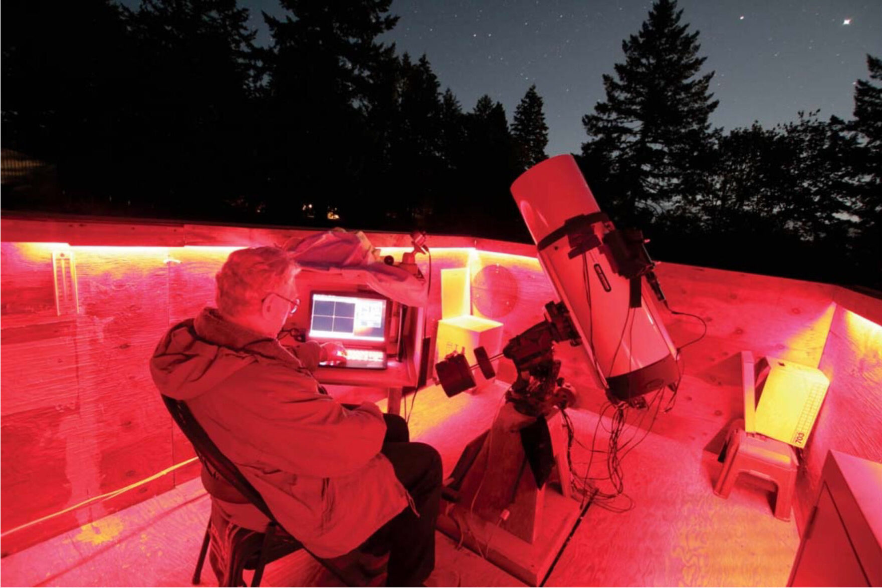
One way we can answer some of these questions is through the process of photometry. This is the art and science of measuring brightness radiated by astronomical objects — a pursuit that a growing number of amateur astronomers is undertaking from backyards, rooftops, balconies, and observatories all over the world. As a science, many amateur astronomers today apply photometry to the study of the most interesting stars: variable ones that change in brightness. Here’s how you can get involved and contribute valuable science yourself.

Analyzing Starlight

These days, we can accurately measure the magnitudes of stars by recording them with digital cameras equipped with CCD or CMOS detectors. These detectors consist of an array of millions of tiny photodiodes packed into a convenient chip package. The camera body provides a safe and clean environment for the light-sensitive chip. It also contains electronics to power the chip, scan its array, and return a digital signal representing the image that fell on the chip.

To capture an image, the telescope focuses light on the sensor in the camera. Although CCDs and CMOS work somewhat differently, the process begins the same way. The camera clears stray charge from the photodiode elements. The chip is then ready to receive photons. During the exposure, photons strike the sensor, generating electrons. When the exposure ends, each photodiode in the array holds a number of electrons proportional to the number of photons that fell on it.

The camera then converts these stored electrons into a digital signal and streams it back to the computer. The computer adds information about the image, such as the width and height of the array, the date, time, length of exposure, as well as any other information needed to document the observation. It then saves the data as a FITS file (a standard astronomical file format).

Calibration Is Key

One fundamental problem we face in making accurate measurements of starlight is that every photodiode on a sensor is slightly different from every other photodiode. These differences are small but measurable. Once captured in an image, the signal coming from a photodiode is called a pixel (short for “picture element”). As captured in a raw image, a pixel might be a fraction of a percent more sensitive than its neighbor, be more affected by noise, or respond to the chip’s temperature a bit differently. The key to making scientifically accurate images is to map these small flaws and correct them.

How is this done? First, we need to quantify all the flaws in the detector. This is accomplished by recording and applying images known as calibration frames, commonly referred to as dark frames and flat-field images.

Dark frames are maps of the small electric current known as dark current that accumulates even when no light is striking the photodiode. They also record the fixed-pattern noise signal from the sensor. Dark frames are created by covering the telescope or closing the camera’s shutter and recording an image with the same duration and at the same temperature as the light images you make of your target stars.

Because dark current varies randomly, we need to take many dark frames and average them together. If I were planning to record 5-minute exposures of my target, I’d also take a few dozen 5-minute dark frames.

The other calibration frame is a flat-field image. This records each photodiode’s sensitivity to light, as well as any variations in the optical train of your telescope, including vignetting or dust motes on any optical element in the light path that can slightly skew the measured result. Typically, these are images of the twilight sky or a uniform light source, such as an electroluminescent panel. Flat-field images also require their own dark frame calibration, which you take using the same exposure you used for the flat frame. These are called dark-flat frames, or sometimes flat darks.

To beat down random variations in these images, an observer typically records multiple dark, flat, and flat-dark frames and then averages each of the results to produce low-noise “master” dark and flat frames.

After a night of imaging, you typically open the images of your target stars in your preferred astronomical imaging program. Depending on your camera, the images may look a bit noisy and mottled with “donut”-shaped dark areas. You then apply your master calibration frames — subtracting the master dark frame to remove dark current, then dividing it by the master flat-frame to correct non-uniformities in the chip and the telescope optics. The resulting calibrated image consists of millions of pixels corrected for the sensor’s quirks and foibles. Each pixel in the image becomes a reasonably faithful record of the light that fell on the corresponding photodiode at the focus of your telescope. Photometrists refer to properly calibrated images as “science frames.”

Astronomers Use Filters

Color is integral to astronomy. The eye sees a narrow range of wavelengths centered at 555 nanometers, in the yellow/green, but stars radiate over a wide range of wavelengths depending on their energy output, temperature, and chemistry. To limit what wavelengths the camera sees, we place carefully defined color filters ahead of the image sensor.

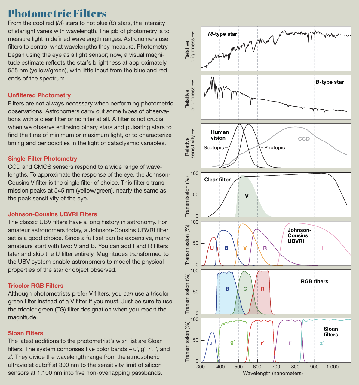
Color filter photometry gave birth to one of the most powerful tools astronomers use: the Hertzsprung-Russell diagram. The diagram shows the absolute magnitude, measured through a V-filter, against the color, measured via the difference between V-filter and B-filter magnitudes, for a range of stars. By plotting an individual star on this diagram, you can glean its relative redness or blueness, clues to its temperature and spectral class. Color photometry reveals which stars are main sequence, blue giants, red giants, red dwarfs, and white dwarfs, and where our Sun fits among them.

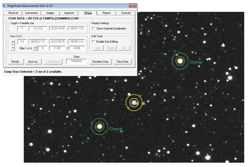
Measuring Magnitudes

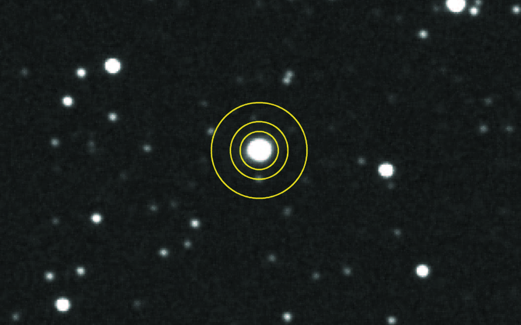
So you have a science image filled with stars. How do you extract the magnitude of a star from an image? Fortunately, most good astronomical image-processing software includes tools to measure the magnitudes of stars. After loading your image into your preferred program, the first task is setting the radii of the measurement tool that you will use to extract magnitude measurements. You can use any star for this. The tool typically has three radius settings. The innermost is the aperture. This should be set to fit tightly around the star you are studying but without cutting off its edges, ideally containing at least 90% of the target stars light. The aperture contains the combined light of the star and its sky background. The second and third radii define an annulus (or “donut”) of sky surrounding the star image. The inner radius of the annulus must be larger than the aperture radius, leaving a gap. The outer annulus radius should be big enough to include a good amount of sky, but small enough to exclude any nearby bright stars. The annulus is used to measure the sky brightness.

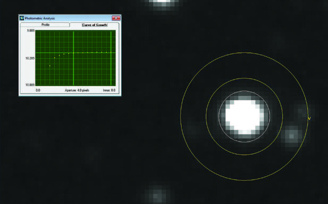
With the radii set, click on a star you wish to measure. The computer surveys the pixels near your click point, finds the brightest ones, and computes a preliminary center for the star image. From that location, an algorithm decides which pixels contain starlight and which do not. It finds the weighted “center of gravity” of the star pixels and finds the exact center of the star image: its centroid.

The aperture you chose appears as a circle with its center aligned at the centroid, surrounded by the inner and outer annulus radii. The software then gets to work counting the number of pixels inside the aperture radius and finds the sum of those pixels. Next, it surveys all the pixels in the annulus. The average value of the annulus pixels is close to the sky brightness, though not exactly because the annulus often includes a few faint stars. The program may take the median value of the annulus pixels, or it may apply a more complex algorithm to find an accurate sky brightness.

The computer’s final step in the process is to subtract the light from the background sky. The trick is this: The computer found the total pixel value in the aperture (star plus sky) and also counted the number of pixels in the aperture. It multiplies the sky background value by the number of aperture pixels, then subtracts the sky total from the star plus sky total. The result is the total pixel value of the star image with no sky light.

Our end goal isn’t a brightness in pixel values, but rather a brightness in the logarithmic scale of stellar magnitudes. The magnitude equation m = –2.5 log10 (S)+Z, converts the linear pixel value sum to an instrumental magnitude, m. In the equation, S is the signal, the sum of star pixels, and Z is the zero-point constant. The zero-point constant is determined by observing standard stars to produce a reasonable apparent magnitude value.

Photometry Made Easy

Differential photometry is the “sweet spot” for amateur astronomers, and my preferred method for as long as I have been doing photometry. This technique measures a star’s brightness relative to a nearby comparison star of known magnitude. For many observing programs, you can ignore atmospheric extinction and transforming instrumental. magnitudes into standard magnitudes. Best of all, differential photometry is a great way to get started doing photometry.

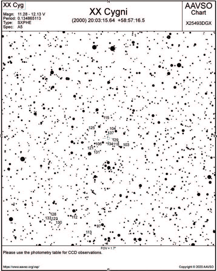
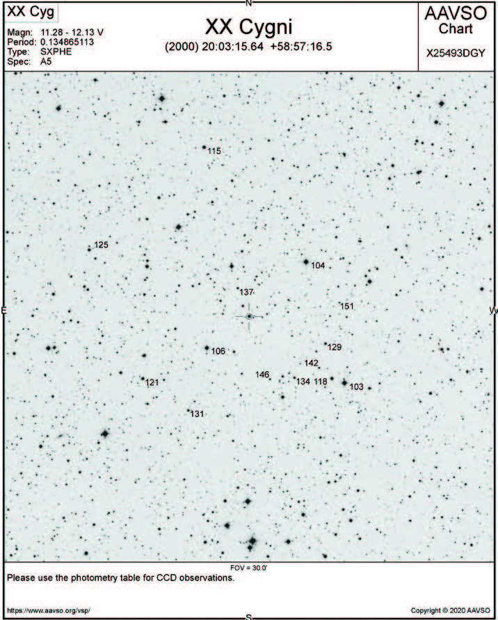
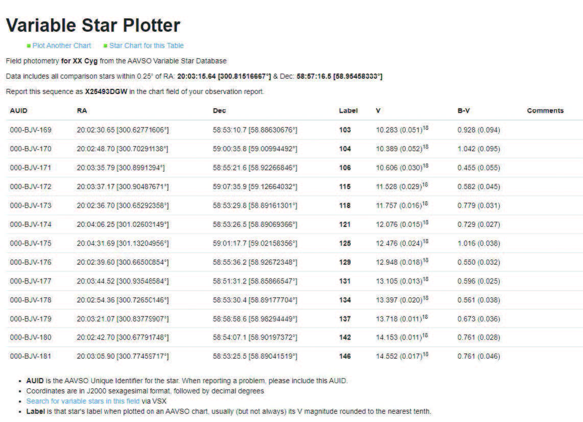
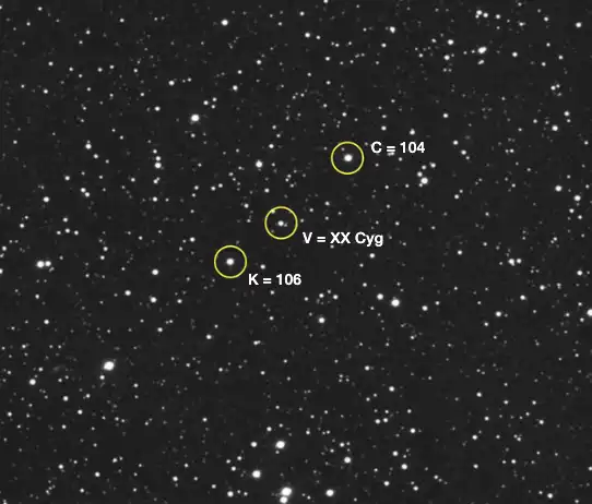
Visiting the American Association of Variable Star Observers (AAVSO) observer page (aavso.org/observers), you’ll find extensive advice about choosing variable star observing programs. Fair warning: It can be overwhelming! But as an example, let’s focus on just one star, one of my favorites: XX Cygni. It’s a pulsating SX Phe star, with a 3.23-hour period and an amplitude of 0.85 magnitude, and it varies enough to see visually in a telescope. You can observe an entire cycle or more in just one night, and for northern observers, it’s high in the sky in summer through late autumn. (A fast variable during the winter months is BL Camelopardis.)

Making a series of variable star observations is just like making sub-exposures for a stacked deep-sky image. For this work, you can use a CCD or CMOS camera (including DSLR and mirrorless models). Be sure to take matching dark and flat frames, or use library master darks and flats to calibrate the images. On each image, extract the instrumental magnitudes of the variable (V), the comparison star (C1), and the “check” star that serves as a second comparison (C2). (We've shown an AAVSO star chart for XX Cygni above, and the figure below shows an image from a time series with XX Cygni as well as a comparison and a “check” star, labeled C and K, respectively.)

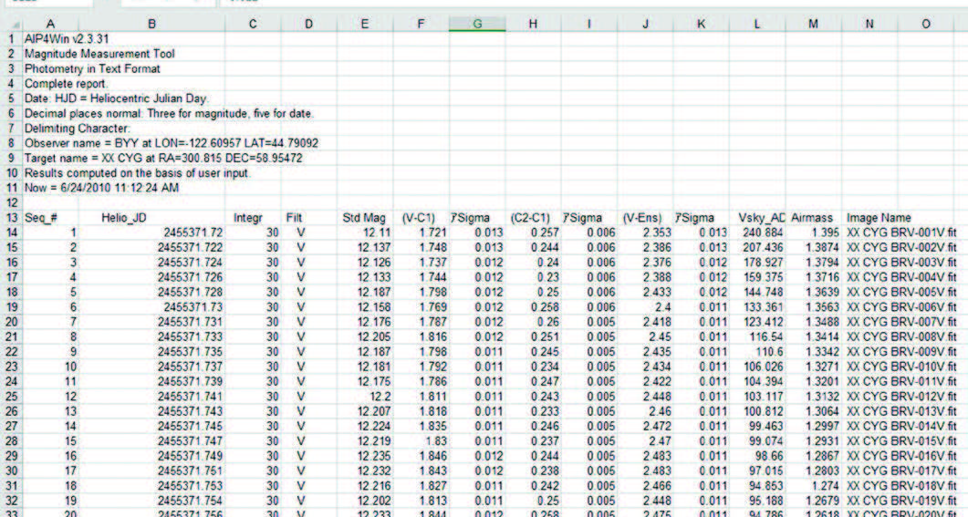
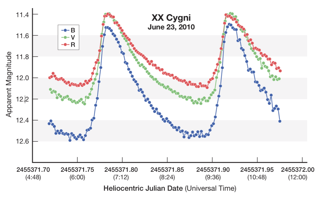
Enter the time each image was made, along with the V, C1, and C2 magnitudes into a spreadsheet program. To find differential magnitude, place the difference between the variable and comparison star in one column and the difference between the check star and the comp star in the other. When you plot them on a graph, the XX Cygni plot rises and falls while the check star plot remains flat. The beauty of this method is that atmospheric extinction is nearly the same for all three stars and cancels out.

For some historical context, search online for “astronomy XX Cygni” to learn how the Harvard astronomer Harlow Shapley made light curves for this star in 1914 and 1915, and see how many other astronomers have studied its slowly changing period of variation.

Correcting Atmospheric Extinction

We Earth-bound observers view stars through our planet’s atmosphere: It acts as a filter, blocking fractions of the star’s light at different wavelengths. The loss is called extinction. In differential photometry, the V star, C1, and C2 suffer nearly equal extinction, so it largely cancels out. However, if your goal is to obtain an accurate magnitude for a star, you must measure the extinction every night and compensate for it.

Astronomers call the depth of atmosphere between the target and the telescope air mass. Straight overhead, the air mass equals 1, or one atmospheric thickness. At 45° from the zenith, starlight passes through 1.4 air masses, and at 60° the air mass reaches 2. Photometrists prefer to avoid working through an air mass greater than 2.5. Many camera-control programs embed the computed air mass in each image’s FITS header.

The observing procedure to measure extinction is simple: As the evening progresses, you measure the instrumental magnitudes of two stars, one rising and the other setting. As the eastern star rises, it brightens; stars in the west dim as they set. Performing this measurement once an hour is often enough. At the end of the night, plot a graph of instrumental magnitude versus the air mass. On a clear night, the plot should be a straight line. The slope of a best-fitting line through the points tells you how much extinction occurs for each air mass — the extinction coefficient — which is typically around 0.2 magnitudes per air mass for a V filter. Corrections get a bit more complicated for very red and very blue stars, where you may encounter non-linear effects.

To correct for extinction, you subtract the air mass of the star times the extinction coefficient from the instrumental magnitude. That gives the star’s magnitude at zero air mass — outside Earth’s atmosphere. Extinction coefficients at high altitude observatories are smaller than those in humid, hazy, and low-altitude continental observing sites, which also often change from night to night.

Transformation to Standard Magnitude

Quite often the goal in photometry is to produce a standard magnitude that can then be compared directly to the magnitudes measured at any other observatory with any other telescope and camera. Just as correcting for atmospheric extinction removes the effects of a star’s location in your sky, transformation to the standard magnitude system corrects the instrumental signature of your telescope and camera. But even though you may be using a set of Johnson-Cousins UBVRI or Sloan filters, minor variations in the filters you use, or the wavelength sensitivity of your camera’s sensor, will introduce small mismatches.

The solution is similar to that for atmospheric extinction: Observe a set of diverse standard stars that have carefully determined U, V, B, R, and I (or Sloan) magnitudes, then determine linear equations that transform your extinction-corrected instrumental magnitudes to the standard system. You first determine the transform coefficients and zero-point for each filter you are using. To do this, image one of several open clusters (such as M67 or M11) or standard fields, then extract the instrumental magnitudes. The AAVSO provides complete instructions and software for recording standard fields, as well as generating coefficient values and applying transforms.

Get Involved

You’ll want to get your feet wet with an observing program of differential photometry as you gain confidence in your newfound knowledge of this rewarding branch of astronomy. Photometry is an excellent pursuit on bright moonlit nights. As you get deeper into it, every night offers an opportunity to find something quite unexpected, as well as the satisfaction of knowing that you’re making a real contribution to astronomy.

Further Reading

• The Handbook of Astronomical Image Processing by Richard Berry and James Burnell. Written for amateur astronomers and includes a copy of AIP4WIN PC software.
• The Sky Is Your Laboratory: Advanced Astronomy Projects for Amateurs by Robert Buchheim. Advice and projects on observing and performing photometry.
• To Measure the Sky: An Introduction to Observational Astronomy by Frederick R. Chromey. An undergraduate college astronomy laboratory textbook.
• The AAVSO Guide to CCD Photometry. A practical guide to getting started.

This article originally appeared in the December 2020 issue of Sky & Telescope.